library(ggplot2)
library(ggthemes)
library(ggrepel)
library(ggspatial)
library(rnaturalearth)
library(rnaturalearthhires)
library(dplyr)
library(readxl)
library(gsheet)Map
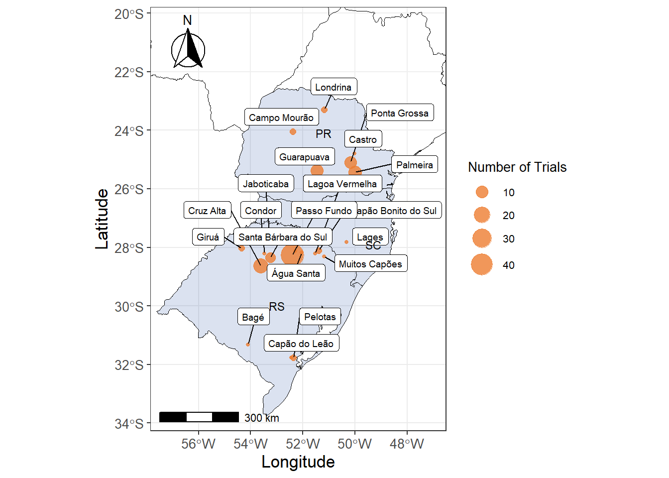
Here’s the code for the map construction.
Libraries
Geographic data
We’re going to upload the trial location data.
# Geographic data
BRA <- ne_states(country = "Brazil", returnclass = "sf")

# Import data
lat_lon <- gsheet2tbl("https://docs.google.com/spreadsheets/d/1MBiKsosQ8Hob6LkS65_1pPU25hx1CO9i42Sm_xf28ww/edit?gid=0#gid=0") |>
    dplyr::select(study, location, state, lat, lon) |>
    filter(study %in% 1:125) |>
  group_by(location) |>
  summarise(
    state = first(state),
    lat   = first(lat),
    lon   = first(lon),
    n_studies = n_distinct(study)  # conta estudos únicos
  ) |>
  ungroup()

lat_lon$lat <- as.numeric(lat_lon$lat)
lat_lon$lon <- as.numeric(lat_lon$lon)

# Define map boundaries based on coordinates
long_min <- min(lat_lon$lon, na.rm = TRUE) - 3.5
long_max <- max(lat_lon$lon, na.rm = TRUE) + 3.5
lat_min <- min(lat_lon$lat, na.rm = TRUE) - 2.5
lat_max <- max(lat_lon$lat, na.rm = TRUE) + 3.5

# Highlight selected states
highlighted_states <- c("PR", "RS", "SC")
BRA$highlight <- ifelse(BRA$postal %in% highlighted_states, "Highlighted", "Normal")

# Label adjustments
nudge_x_vals <- ifelse(lat_lon$location == "Água Santa", -0.1, 0.5)
nudge_y_vals <- ifelse(lat_lon$location == "Água Santa", -0.5, 0.7)
Build the map
Here, we’re going to build the map using the ggplot2 package.
# Build the map
main_map <- ggplot(BRA) +
  geom_sf(aes(fill = highlight), alpha = 0.2, color = "black") +
  scale_fill_manual(values = c("Highlighted" = "#4970b5", "Normal" = "white"), guide = "none") +
  geom_point(data = lat_lon, aes(lon, lat, size = n_studies), alpha = 0.8, color = "#ed7d31") +
  coord_sf(xlim = c(long_min, long_max), ylim = c(lat_min, lat_max), expand = FALSE) +
  geom_label_repel(data = lat_lon,
                   aes(lon, lat, label = location),
                   size = 2.5,
                   nudge_x = nudge_x_vals,
                   nudge_y = nudge_y_vals,
                   fill = "white", color = "black",
                   max.overlaps = Inf) +
  scale_size_continuous(range = c(1, 8), guide = guide_legend(title = "Number of Trials")) +
  labs(x = "Longitude", y = "Latitude") +
  theme_bw() +
  theme(axis.title.y = element_text(size = 13),  # enable Markdown in Y-axis label
    axis.title.x = element_text(size = 13),
    axis.text.x = element_text(size = 10),
    axis.text.y = element_text(size = 10),
    legend.position = "right", text = element_text(size = 10)) +
  annotation_scale(location = "bl", width_hint = 0.3) +
  annotation_north_arrow(location = "tl", which_north = "true",
                         style = north_arrow_fancy_orienteering()) +
  annotate("text", x = -51.2, y = -24.1, label = "PR", size = 3, color = "black") +
  annotate("text", x = -53, y = -30, label = "RS", size = 3, color = "black") +
  annotate("text", x = -49.3, y = -27.9, label = "SC", size = 3, color = "black")
Map visualization
main_map